You are invited to first read the first paragraph of the page “The Yellow Scale”.
In the present page “libration” stands for “longitudinal libration”.
The system Earth Moon is supposed isolated.
Why and how?
The two main observations concerning the Moon rotation have been known for ages. They are first the dark side and second the libration.
The first one has been addressed in the page “The Yellow Scale”. The second one will be addressed hereunder by means of a simulation.
The most common explanation of a white (spinning) Moon libration is kinematic, by a mix of its spin and the eccentricity of its orbit. Obviously it cannot apply to a yellow (not spinning) Moon which requires instead a mechanics explanation: the libration is due to an imbalance in the mass distribution of the Moon or/and an oval form due to tidal forces.
The simulation model is the simplest of all: it supposes that all the imbalance of the Moon is concentrated in a high density spot (a kind of mini black hole) situated at the bright pole (often called the near side) of the Moon, the latter being supposed perfectly spherical.
Mapping
The mapping is the lay out of the figures involved: axes, lines, points, angles. It is refreshed every sample (calculation loop).
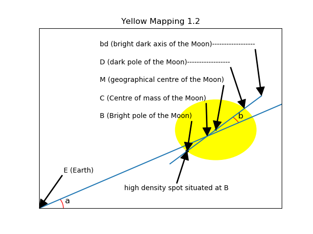
All events unfold in the plane of a lunar orbit, with a Moon rotating on an axis supposed perpendicular to that plane.
The reference frame is defined by 2 perpendicular axes, the origin of which is the center of the Earth E (confounded with the center of mass of the system Earth/Moon). At start, its x axis points to the center of mass of the Moon M.
A second frame, relative to the Moon, is defined by an axis named bd which enters at the bright pole (0,0) and exits at the dark pole(0,180).
The origin of bd is the center of mass of the Moon C. bd pivots around C according to the said pendulum movement.
The angle between the x axis and EC is labelled a. It is always positive (counter clockwise).
The angle between EC and bd is labelled b. It oscillates around 0. It is maximum and positive at start.
Program in Python 3.7
It can be understood and run without knowing Python because it is so clear a language.
The computing environment is reduced to a minimum. The only rule needed is to copy Python 3 and all the imported modules in the same path (directory). You can use the terminal but an editor such as sublime text is preferred.
Try to paste directly the code which follows to your editor. When I do this with mine (Sublime Text), not only does the program run fine, but moreover the editing is dramatically improved: not a single line is cut.
Don’t forget to recompile after pasting. In my pc this translates into:
ctrl + S for compilation followed by ctrl + B for launching.
The output is a figure build up with the Matplotlib library.
The position of the Moon (angle a) and its libration (angle b) are shown every nb_samp_between_plots samples (typically 20) all along one orbit.
The basic result
Image obtained with libration = 1
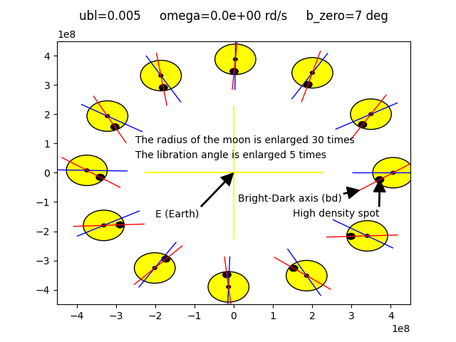
The simulation shows that it is necessary to choose an imbalance of 0.005 to find the observed longitudinal libration, i.e. one oscillation per lunar orbit.
If the imbalance of the Moon was concentrated at the Bright crater its relative value would be 0.005.
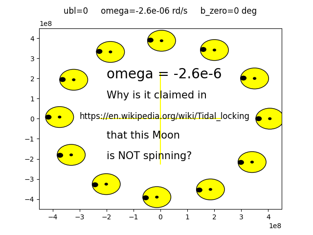
Results in “rotation” mode
The value of any parameter is to be changed directly in the program, there is no formalized entry. This is very flexible but it implies to recompile after any modification.
So the program can be used to reproduce as faithfully as possible the animated figures located at the top of the page of the site https://en.wikipedia.org/wiki/Tidal_locking.
We then find by simulation the fact demonstrated by the geometry in the chapter “The yellow scale”, namely: the legend relating to the animated figures is erroneous, it is the right Moon which turns on itself and not the one on the left.
Image obtained with libration = 0 and “rotation” = “left”:
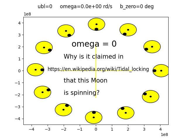
Image obtained with libration = 0 and “rotation” = “right”:
Code
# coding = utf - 8

"""
                           ********************************************************
                           * SIMULATION OF THE LONGITUDINAL LIBRATION OF THE MOON *
						   *				   28 february 2022 				  *
                           ********************************************************


MAIN PURPOSE OF THE PROGRAM: libration mode

This program is essentially intended for the simulation of the longitudinal libration of a yellow moon.
(which does not rotate).
The libration is due to an inhomogeneity in the mass of the Moon which causes by tumble effect an
oscillation of about 7 degrees per lunar orbit.
To highlight the phenomenon it is chosen the simplest possible mass distribution: that of a homogeneous
moon with a very small region of very high density at the closest point to the Earth
causing an imbalance whose relative value is measured by the variable ubl.
The simulation shows that the calculated libration is equal to the real one for a value of ubl equal
to 5 per thousand.


SECONDARY PURPOSE OF THE PROGRAM: rotation mode

The program can also be used to reproduce as faithfully as possible the animated figures located at
the top of the page of the site https://en.wikipedia.org/wiki/Tidal_locking.
We then find by simulation the fact demonstrated by the geometry in the chapter "The yellow scale",
namely: the legend relating to the animated figures is erroneous, it is the right Moon which turns on
itself and not the one on the left.
You can switch from one mode to the other by manually changing the 2 flags libration and rotation of the
2 first active lines of the program.


NOTATIONS AND LABELLING OF THE VARIABLES:  *************************************************

the vectors begin with an upper case letter.
the vector from B to C is labelled BC. But, as E is the origin, the vector EC is labelled C.
the scalars begin with a lower case letter.
the coordinates of the point P are those of the vector EP (because E is the origin of the plan).
the distance between the points B and C is labelled lBC (l stands for length).
the unit vector of an axis begins with the upper case U.
the angles are expressed  1/in radians for calculations  2/ in degrees for inputs/outputs (with suffix _d).
"""


libration = 1										#0: rotation mode		1: libration mode
rotation = "left"										#"left": related to the left animated figure
													#"right": related to the right animated figure

if libration == 1 and rotation == "right":				#just to be sure that omega is set to
	rotation = "left"									#0 when libration is set to 1


import numpy as np
import matplotlib.pyplot as plt
import math
import matplotlib.lines as lines

import matplotlib.path as path
import matplotlib.patches as patches


pi = math.pi  ;  sqrt = math.sqrt  ;  cos = math.cos  ;  sin = math.sin


#FUNCTIONS *********************************************************************************

def sum(V0,V1):                                     #sum of vectors V0 and V1
    return V0[0] + V1[0], V0[1] + V1[1]
def mod(V):                                         #module of the vector V
    return sqrt(V[1]**2 + V[0]**2)
def kV(k, V0):                                      #product of vector V0 by a scalar k
    return k*V0[0], k*V0[1]
def Vecprod(V0, V1):                                #scalar of the vectorial product of vectors V0 and V1
    return V0[0]*V1[1] - V0[1]*V1[0]
def unit(V):                                        #unitary Vector of an axis bearing (parallel to)
    return kV(1/mod(V), V)                              #the vector V


#UNIVERSAL CONSTANTS  *********************************************************************

r = 1.737e6                         #radius of the Moon (m)
mass = 7.34e22                      #mass of the Moon
mass_earth = 5.97e24                #mass of the Earth
g = 6.673e-11                       #gravitational constant  N·(m/kg)
v_zero = 970                        #velocity of the Moon at start (m/s)
lEC_zero = 4.06e8                   #Distance (length) at start between the mass centre C
                                    #    of the Moon and the Earth M (at apogee).
                                    #As regards the distance between Earth and Moon,
                                    #    EC and EM are supposed equal.

                                    #https://en.wikipedia.org/wiki/Lunar_distance_(astronomy)
                                    #from 356,500 km at the perigee to 406,700 km at apogee,
                                    #https://nssdc.gsfc.nasa.gov/planetary/factsheet/moonfact.html
                                        #Perigee            3.63e8
                                        #Apogee              4.06e8  **************
                                        #Max. orbital velocity     1082
                                        #Min. orbital velocity (km/s)    0.970  **********
                                        #revolution period (days)    27.3217


#CONSTANTS

ubl = + .005                        #relative unbalance due to the HDS (high density spot)
if libration == 0: ubl = 0
mass_s = ubl*mass                   #mass of the HDS
da = .01                            #angular orbital increment of a sample (rd)
b_zero_d = 7						#pendulum angle of the Moon at start IN DEGREES
if libration == 0: b_zero_d = 0
b_zero = b_zero_d*pi/180            #pendulum angle of the Moon at start (in rd of course)

m = mass_s*r/(mass)                 #abciss on the axis bd of the geographic centre of the moon
                                    #bd is the relative axis joining the bright and dark poles.
                                    #bd is oriented from bright pole to dark pole.
                                    #Its origin is C, center of mass of the Moon.

s = - r                             #abciss on the bd axis of the HDS

I = mass*r**2*(1 + ubl)             #moment of inertia (relative to C) of the Moon


#FOR VISUALIZATION NEEDS

kb = 5                              #ampli factor applied on the pendulum angle for visu needs
if libration == 0: kb = 1
kr = 30                             #ampli factor applied on the radius for visu needs
r_v = kr*r							#radius of the visualized Moon
rspot_v	= r_v/5						#radius of the visualized HDS
									#recall: the real HDS has no radius. It is infinitely small
s_v = -r_v + rspot_v				#abcissis on the bd axix of the centre of the visualized HDS


#INITIALIZATION OF THE VARIABLES   ********************************************************

a = 0                               #orbital angle at start (rd)
b = b_zero                          #pendulum angle at start (rd)
if libration == 0: b = 0
omega = 0                           #angular velocity of the Moon around its centre of mass (rd/s)
									#(omega = dbeta/dt)

if rotation == "right": omega = -2*pi/(28*24*3600)
C = [lEC_zero, 0]                   #vector EC (coordinates of the centre of mass of the Moon (m))
V = [0, v_zero]                     #coordinates of the vector velocity of the centre of mass (m/s)
t = 0                               #time
dt = da*lEC_zero/v_zero             #time orbital increment of a sample.
                                    #dt is not constant. This is only its initialization value.
                                    #dt is NOT the increment of the main loop.
                                    #dt is calculated at each loop. The true increment is angle da.
nb_samp_total = int(2*pi/da)        #number of samples of the MAIN LOOP
nb_plots = 12                       #number of plots of the MAIN LOOP
nb_samp_between_plots = int(nb_samp_total/nb_plots)          #number of samples between 2 plots


#GRAPHICS  (except the plotting of the Moon itself)*****************************************

fig = plt.figure(figsize=(7, 6))	#total size: 7 by 6 inches
ax = fig.add_subplot(1,1,1)

xy = 450e6
xmin =  - xy  ;  xmax = xy  ;  ymin =  - xy  ;  ymax = xy
segment = lEC_zero/10   #should rather be in MAIN LOOP but is here because it is a fixed value.
s1="{:.1e}".format(omega)
titre1 = 'ubl=' + str(ubl) + '     omega=' + s1 + ' rd/s' + '     b_zero=' + str(b_zero_d) + ' deg' + '\n'
ax.set(xlim = (xmin, xmax), ylim = (ymin, ymax), title = titre1)
plt.plot([xmin/2, xmax/2], [0,0], color='yellow')  ;  plt.plot([0,0], [ymin/2, ymax/2], color='yellow')

def annot(txt, xy, xytext):
	ax.annotate(txt, xy, xytext, arrowprops=dict(facecolor='black', shrink=0.01, width=1))
def annot1(txt, xy, size):#**kwargs):
	ax.annotate(txt, xy, size=size)

if libration == 1:
	annot('E (Earth)', (0, 0), (-2e8, -1.5e8))
	annot1('The radius of the moon is enlarged ' + str(kr) + ' times', (-2.5e8, 1e8), size=10)
	annot1('The libration angle is enlarged ' + str(kb) + ' times', (-2.5e8, .5e8), size=10)
if libration == 0:
	if rotation == "left":
		annot1('omega = 0', (-1.5e8, 2e8), size=20)
		annot1('Why is it claimed in', (-2e8, 1e8), size=15)
		annot1('https://en.wikipedia.org/wiki/Tidal_locking', (-3e8, 0), size=12)
		annot1('that this Moon', (-2e8, -1e8), size=15)
		annot1('is spinning?', (-2e8, -2e8), size=15)
	if rotation == "right":
		annot1('omega = -2.6e-6', (-2e8, 2e8), size=20)
		annot1('Why is it claimed in', (-2e8, 1e8), size=15)
		annot1('https://en.wikipedia.org/wiki/Tidal_locking', (-3e8, 0), size=12)
		annot1('that this Moon', (-2e8, -1e8), size=15)
		annot1('is NOT spinning?', (-2e8, -2e8), size=15)


#MAIN LOOP  ********************************************************************************
           #********************************************************************************


for i_sample in range(nb_samp_total):


	def mapping1():                        #see figure 2 (geometric mapping)

		global lEC, lEB, Ue, Ufs, Um, M, Umm, B
		Ue = (cos(a), sin(a))                     #unitary vector on the axis EM
		Um = (cos(a + b), sin(a + b))             #unitary vector on the axis bd
		Umm = (cos(a + kb*b), sin(a + kb*b))      #unitary vector on the axis bd "magnified" (displayed)
		M = C                              #centre of the Moon
		CB = kV(s, Um)                     #vector CB
		B = sum(C, CB)                     #vector EB: coordinates of the point B
		Ufs = unit(kV(-1, B))              #unitary vector of the attractive force due to the HDS.
		lEC = mod(C)                       #distance between the Earth and the centre of mass of the Moon
		lEB = mod(B)                       #distance between the Earth and the HDS (or B)


	mapping1()


    #TRAJECTORY OF THE CENTRE OF MASS OF THE MOON

	f = g*mass*mass_earth/lEC**2
	F = kV(-f, Ue)  ;  fx = F[0] ;  fy = F[1]
	V = sum(V, kV(dt/mass, F))
	C = sum(C, kV(dt, V))


    #PENDULUM MOVEMENT

	fs = g*mass_s*mass_earth/lEB**2     #module of the force exercised by the Earth on the HDS
	Fs = kV(fs, Ufs)                    #vector of the force exercised by the Earth on the HDS
	moment = Vecprod(kV(s, Um), Fs)     #scalar of the moment due to the HDS


    #OUTPUTS

	if (i_sample % nb_samp_between_plots  == 0) and (i_sample < (nb_samp_total -10)):
		gamma = b*180/pi                        #gamma in degrees
		MB_v = kV(s_v, Umm)						#visualized vector MB
		B_v = sum(M, MB_v)                      #coordinates of the centre of the visualized HDS
		moon = patches.Circle(M, r_v, alpha=1, facecolor="yellow", edgecolor="black")
		spot = patches.Circle(B_v, rspot_v, alpha=1, color="black")
		centre = patches.Circle(M, r_v/10, alpha=1, color="black")
		me1 = sum(M, kV(-2*r_v, Ue))  ;  me2 = sum(M, kV(1.5*r_v, Ue))
		bd1 = sum(M, kV(-2*r_v, Umm))  ;  bd2 = sum(M, kV(1.5*r_v, Umm))
		axis_me1 = (me1, me2)
		axis_bd1 = (bd1,bd2)
		axis_me = patches.Polygon(axis_me1, color="blue")
		axis_bd = patches.Polygon(axis_bd1, color="red")
		ax.add_artist(moon)
		ax.add_artist(spot)
		ax.add_artist(centre)
		if libration == 1: ax.add_artist(axis_me)  ;  ax.add_artist(axis_bd)

		if  libration == 1 and i_sample == 0:
			annot('Bright-Dark axis (bd)', bd1, (.1e8, -1e8))
			annot('high density spot (HDS)', B_v, (.1e8, -1.5e8))


	mapping1()


    #INCREMENTATIONS

	v_trajectory = sqrt(mod(V)**2)
	dt = da*lEC/v_trajectory
	a = a + da
	b = b + omega*dt
	omega = omega + moment*dt/I
	t = t + dt


#FINAL

days = t / (24*3600)
print ('\n', i_sample, '   ', 'v0=', v_zero, '    ', 'total time=', '%.2f' % days,'days')

plt.show()